本帖最后由 levycui 于 2017-12-13 15:00 编辑
问题导读:
1、如何将对象放入计算图运算?
2、创建一个numpy数组?
3、如何在同一个计算图上进行多个操作?
4、数据在经过分层时如何改变?

上一篇:TensorFlow ML cookbook 第一章7、8节 实现激活功能和使用数据源
张量流的方式
在本章中,我们将介绍TensorFlow如何操作的关键组件。 然后我们将它们联系起来,创建一个简单的分类器并评估结果。 在本章末尾,您应该了解以下内容:
- 计算图中的运算
- 分层嵌套操作
- 使用多个图层
- 实施损失函数
- 实施向后传播
- 使用批量和随机培训
- 把一切结合在一起
- 评估模型
介绍
现在我们已经介绍了TensorFlow如何创建张量,使用变量和占位符,我们将介绍如何在计算图中对这些对象进行操作。 由此,我们可以建立一个简单的分类器,看看它的表现如何。
计算图中的运算
现在我们可以将对象放入我们的计算图中,我们将介绍对这些对象起作用的操作。
准备
要开始一个图表,我们加载TensorFlow并创建一个会话,如下所示:
[mw_shl_code=python,true]import tensorflow as tf
sess = tf.Session()[/mw_shl_code]
如何做
在这个例子中,我们将把我们所学到的东西和列表中的每个数字都加入到一个图表中的操作中,然后打印输出:
首先我们宣布我们的张量和占位符。 在这里,我们将创建一个numpy数组来馈入我们的操作:
[mw_shl_code=python,true]import numpy as np
x_vals = np.array([1., 3., 5., 7., 9.])
x_data = tf.placeholder(tf.float32)
m_const = tf.constant(3.)
my_product = tf.mul(x_data, m_const)
for x_val in x_vals:
print(sess.run(my_product, feed_dict={x_data: x_val}))
3.0
9.0
15.0
21.0
27.0[/mw_shl_code]
如何运行
步骤1和2在计算图上创建数据和操作。 然后,在步骤3中,我们通过图形输入数据并打印输出。 这里是计算图的样子:

图1:在这里我们可以看到在图中,占位符x_data和我们的乘法常数一起进入乘法运算。
分层嵌套操作
在这个配方中,我们将学习如何在同一个计算图上进行多个操作。
准备
知道如何将运营连锁在一起非常重要。 这将在计算图中设置分层操作。 为了演示,我们将乘以两个矩阵占位符,然后执行加法。 我们将以三维numpy数组的形式输入两个矩阵:
[mw_shl_code=python,true]import tensorflow as tf
sess = tf.Session()[/mw_shl_code]
如何做
注意数据在经过时会如何改变也很重要。 我们将生成两个大小为3x5的numpy数组。 我们将每个矩阵乘以一个大小为5x1的常量,这将导致一个大小为3x1的矩阵。 然后我们将乘以1x1矩阵再次产生一个3x1矩阵。 最后,我们在最后添加一个3x1矩阵,如下所示:
1.首先我们创建要导入的数据和相应的占位符:
[mw_shl_code=python,true]my_array = np.array([[1., 3., 5., 7., 9.],
[-2., 0., 2., 4., 6.],
[-6., -3., 0., 3., 6.]])
x_vals = np.array([my_array, my_array + 1])
x_data = tf.placeholder(tf.float32, shape=(3, 5)) [/mw_shl_code]
2.接下来我们创建用于矩阵乘法和加法的常量:
[mw_shl_code=python,true]m1 = tf.constant([[1.],[0.],[-1.],[2.],[4.]])
m2 = tf.constant([[2.]])
a1 = tf.constant([[10.]])
[/mw_shl_code]
3.现在我们声明操作并将它们添加到图中:
[mw_shl_code=python,true]prod1 = tf.matmul(x_data, m1)
prod2 = tf.matmul(prod1, m2)
add1 = tf.add(prod2, a1) [/mw_shl_code]
4.最后,我们通过图表来提供数据:
[mw_shl_code=python,true]for x_val in x_vals:
print(sess.run(add1, feed_dict={x_data: x_val}))
[[ 102.]
[ 66.]
[ 58.]]
[[ 114.]
[ 78.]
[ 70.]] [/mw_shl_code]
如何运行
我们刚刚创建的计算图可以用Tensorboard进行可视化。 TensorFlow是TensorFlow的一个特性,它允许我们可视化该图中的计算图和值。 与其他机器学习框架不同,这些功能是本地提供的。 要了解如何完成,请参阅第11章“更多TensorFlow”中的Tensorboard recipe中的可视化图。 以下是我们的分层图形:

图2:在这个计算图中,你可以看到数据的大小,因为它通过图形向上传播。
参考更多
在我们通过图表运行数据之前,我们必须声明数据的形状并知道操作的结果形状。 这并非总是如此。 可能有一两个我们事先不知道或可能会有所不同的维度。 要做到这一点,我们指定可以改变或未知的维度是没有价值的。 例如,要使先前的数据占位符的列数量未知,我们将编写以下行:
[mw_shl_code=python,true]x_data = tf.placeholder(tf.float32, shape=(3,None)) [/mw_shl_code]
这允许我们打破矩阵乘法规则,并且我们仍然必须遵守乘法常数必须具有相同的相应行数的事实。 我们可以动态生成这个数据,也可以在我们的图形中输入数据的时候重新生成x_data。 在后面的章节中,我们分批提供数据时,这将会派上用场。
原文:
The TensorFlow Way
In this chapter, we will introduce the key components of how TensorFlow operates. Then we will tie it together to create a simple classifier and evaluate the outcomes. By the end of the chapter you should have learned about the following:
- Operations in a Computational Graph
- Layering Nested Operations
- Working with Multiple Layers
- Implementing Loss Functions
- Implementing Back Propagation
- Working with Batch and Stochastic Training
- Combining Everything Together
- Evaluating Models
Introduction
Now that we have introduced how TensorFlow creates tensors, uses variables and placeholders, we will introduce how to act on these objects in a computational graph. From this, we can set up a simple classifier and see how well it performs.
Operations in a Computational Graph
Now that we can put objects into our computational graph, we will introduce operations that act on such objects.
Getting ready
To start a graph, we load TensorFlow and create a session, as follows:
import tensorflow as tf
sess = tf.Session()
How to do it…
In this example, we will combine what we have learned and feed in each number in a list to an
operation in a graph and print the output:
1. First we declare our tensors and placeholders. Here we will create a numpy array to
feed into our operation:
import numpy as np
x_vals = np.array([1., 3., 5., 7., 9.])
x_data = tf.placeholder(tf.float32)
m_const = tf.constant(3.)
my_product = tf.mul(x_data, m_const)
for x_val in x_vals:
print(sess.run(my_product, feed_dict={x_data: x_val}))
3.0
9.0
15.0
21.0
27.0
How it works…
Steps 1 and 2 create the data and operations on the computational graph. Then, in step 3, we feed the data through the graph and print the output. Here is what the computational graph looks like:

Figure 1: Here we can see in the graph that the placeholder, x_data, along with our multiplicative constant, feeds into the multiplication operation.
Layering Nested Operations
In this recipe, we will learn how to put multiple operations on the same computational graph.
Getting ready
It's important to know how to chain operations together. This will set up layered operations in the computational graph. For a demonstration we will multiply a placeholder by two matrices and then perform addition. We will feed in two matrices in the form of a three-dimensional numpy array:
import tensorflow as tf
sess = tf.Session()
How to do it…
It is also important to note how the data will change shape as it passes through. We will feed in two numpy arrays of size 3x5. We will multiply each matrix by a constant of size 5x1, which will result in a matrix of size 3x1. We will then multiply this by 1x1 matrix resulting in a 3x1 matrix again. Finally, we add a 3x1 matrix at the end, as follows:
1.First we create the data to feed in and the corresponding placeholder:
my_array = np.array([[1., 3., 5., 7., 9.],
[-2., 0., 2., 4., 6.],
[-6., -3., 0., 3., 6.]])
x_vals = np.array([my_array, my_array + 1])
x_data = tf.placeholder(tf.float32, shape=(3, 5))
2.Next we create the constants that we will use for matrix multiplication and addition:
m1 = tf.constant([[1.],[0.],[-1.],[2.],[4.]])
m2 = tf.constant([[2.]])
a1 = tf.constant([[10.]])
3.Now we declare the operations and add them to the graph:
prod1 = tf.matmul(x_data, m1)
prod2 = tf.matmul(prod1, m2)
add1 = tf.add(prod2, a1)
4.Finally, we feed the data through our graph:
for x_val in x_vals:
print(sess.run(add1, feed_dict={x_data: x_val}))
[[ 102.]
[ 66.]
[ 58.]]
[[ 114.]
[ 78.]
[ 70.]]
How it works…
The computational graph we just created can be visualized with Tensorboard. Tensorboard is a feature of TensorFlow that allows us to visualize the computational graphs and values in that graph. These features are provided natively, unlike other machine learning frameworks. To see how this is done, see the Visualizing graphs in Tensorboard recipe in Chapter 11, More with TensorFlow. Here is what our layered graph looks like:

Figure 2: In this computational graph you can see the data size as it propagates upward through the graph.
There's more…
We have to declare the data shape and know the outcome shape of the operations before we run data through the graph. This is not always the case. There may be a dimension or two that we do not know beforehand or that can vary. To accomplish this, we designate the dimension that can vary or is unknown as value none. For example, to have the prior data placeholder have an unknown amount of columns, we would write the following line:
x_data = tf.placeholder(tf.float32, shape=(3,None))
This allows us to break matrix multiplication rules and we must still obey the fact that the multiplying constant must have the same corresponding number of rows. We can either generate this dynamically or reshape the x_data as we feed data in our graph. This will come in handy in later chapters when we are feeding data in multiple batches.
|

 /2
/2 

 提升卡
提升卡 置顶卡
置顶卡 沉默卡
沉默卡 喧嚣卡
喧嚣卡 变色卡
变色卡 千斤顶
千斤顶 显身卡
显身卡